PART 1 TASK 3: CREATING PIVOT TABLES & GENERATING BUSINESS INSIGHTS

INSTRUCTIONS:

A. Create Two Pivot Tables

1. a. Navigate to the “Task 3-CREATING PIVOT TABLES" tab in the spreadsheet. Review the data in columns A-E 

   b. Use the data you've reviewed to answer the questions below. Place your answers in the "Your Responses" tab of the Google Sheet.

   c. Create the following two pivot tables directly in this tab

1. Pivot Table 1: Total Sales by Month & Store Location and Product Category

   a. Step 1: Select Your Data: Click and drag to highlight the entire dataset you want to summarize (including the headers), 

   b. Step 2: Insert the Pivot Table

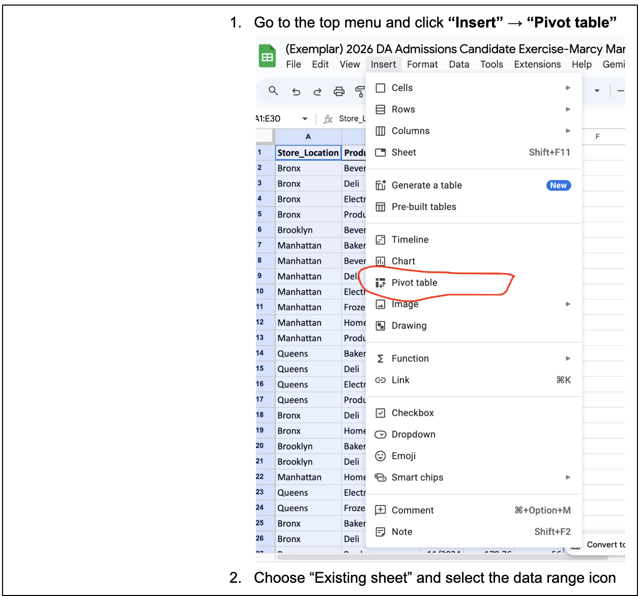
b. Go to the top menu and click “Insert” → “Pivot table”

c. Choose “Existing sheet” and select the data range icon

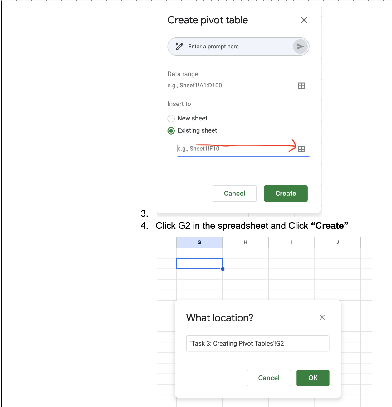
d. Click on the “G2” cell in the spreadsheet and Click “Create”

e. A Pivot Table Editor will appear on the right.

• Click “Add” next to Rows

• Choose the following fields: Product Category and Store Location

• Click “Add” next to Columns

• Choose the following field: Months

• Click “Add” next to Values

• Choose the following field: Total Sales

• Make sure the default summarizes the data correctly by SUM

2. Pivot Table 2: Total Units Sold by Month & Product Category

a. Step 1: Select Your Data: Click and drag to highlight the entire dataset you want to summarize (including the headers), or click into any cell within the dataset if it’s continuous

b. Step 3: Insert the Pivot Table

1. Go to the top menu and click “Insert” → “Pivot table”

2. Choose “Existing sheet” and select “G39” cell. Click “Create”

3. A Pivot Table Editor will appear on the right.

• Click “Add” next to Rows

  • Choose the following fields: Product Category

• Click “Add” next to Columns

• Choose the following field: Months

• Click “Add” next to Values

  • Choose the following field: Units Sold

• Make sure the default summarizes the data correctly by SUM

B. Perform Targeted Calculations

Answer the following questions in the “Response Tab” using data from the pivot tables.

1. Modeling a Sales Drop:

   a. If Manhattan’s Produce sales in August dropped by 30% due to a supply shortage, what would be the new total sales amount for that entry?

2. Estimating Compounding Growth:

   a. Suppose Bakery sales increase by 10% month-over-month, beginning in April, what would be the total Bakery sales from May to December under this growth scenario?

Record your calculations clearly in your workbook or a separate response tab.

C. Analyze & Interpret Trends

Use your pivot tables to answer the following questions. These are not just number-based — they’re about observing patterns and reasoning through what they might mean for the business.

3. Category Momentum” Which product category appears to gain the most momentum (growth in units sold) over the year? What might be driving that trend

4. Borough-by-Borough Breakdown: Which borough appears to perform unusually well in one product category? Why might this be

5. Units vs. Revenue: Choose a category where the units sold are high, but the total sales are relatively low. What does this tell you about the average price point and what might the business do in response?